Contents

% DEMO_01_INTRODUCCION Guía Práctica e Introducción a Modelos Dinámicos
% Curso guiado de GSUA-CSB
%
% Este script proporciona una introducción pedagógica a la formulación de
% modelos en tiempo discreto y continuo definidos por el usuario,
% declarando explícitamente factores (parámetros + condiciones iniciales)
% y nombres de salidas, así como exploraciones de ensamble de incertidumbre.

1. Configuración del Entorno

clc; clear; close all;

% --- Localización portable de la toolbox GSUA-CSB ---------------------------
% Si la toolbox ya está instalada como .mltbx, sus funciones están en el path y
% no hay que hacer nada. Si no, intentamos ubicaciones habituales (sin
% codificar el nombre de usuario) y, si tampoco aparece, DETENEMOS con un
% mensaje claro en vez de fallar silenciosamente más adelante.
if isempty(which('gsua_dataprep'))
    candidatos = {
        fullfile(fileparts(mfilename('fullpath')), '..', '..', '..', 'Functions')  % dentro del repo clonado
        fullfile(getenv('USERPROFILE'), 'MATLAB Drive', 'Toolbox', 'Functions')
        fullfile(getenv('USERPROFILE'), 'Documents', 'MATLAB', 'GSUA-CSB', 'Functions')
    };
    for k = 1:numel(candidatos)
        if isfolder(candidatos{k}), addpath(candidatos{k}); break; end
    end
    if isempty(which('gsua_dataprep'))
        error(['No se encontró la toolbox GSUA-CSB en el path de MATLAB. ' ...
               'Instala GSUA-CSB.mltbx o añade su carpeta Functions con addpath(...).']);
    end
end

% Los modelos de este módulo (discrete_logistic_userdefined,
% sir_continuous_userdefined) viven junto a este script: ruta relativa portable.
addpath(fileparts(mfilename('fullpath')));

fprintf('=========================================================================\n');
fprintf('  MÓDULO 01: INTRODUCCIÓN A MODELOS EN TIEMPO DISCRETO Y CONTINUO  \n');
fprintf('=========================================================================\n\n');

=========================================================================
  MÓDULO 01: INTRODUCCIÓN A MODELOS EN TIEMPO DISCRETO Y CONTINUO  
=========================================================================

2. MODELO 1: TIEMPO DISCRETO (Crecimiento Logístico)

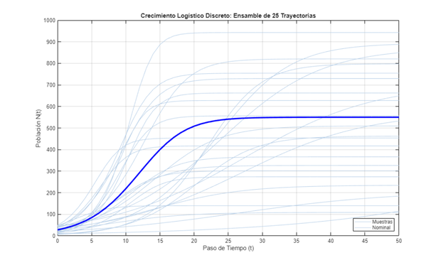
fprintf('--- 1. MODELO LOGÍSTICO DISCRETO ---\n');
fprintf('Ecuación: N(t+1) = N(t) + r * N(t) * (1 - N(t) / K)\n\n');

% Definición de rangos para Factores: [Parámetros + Condición Inicial]
%   Fila 1: r  (tasa de crecimiento)
%   Fila 2: K  (capacidad de carga)
%   Fila 3: N0 (población inicial en t=0)
ranges_discrete = [
    0.05, 0.50;  % r
    100,  1000;  % K
    5,    50     % N0 (Condición inicial)
];

domain_discrete = [0, 50]; % 50 pasos discretos

% Especificación explícita de nombres de factores y nombres de salidas
factor_names_discrete = {'r', 'K', 'N0'};
out_names_discrete    = {'Poblacion'};

[T_discrete, ~] = gsua_dataprep('discrete_logistic_userdefined', ranges_discrete, ...
    'domain', domain_discrete, ...
    'names', factor_names_discrete, ...
    'out_names', out_names_discrete);

disp('Tabla Resumen del Modelo Discreto (Factores y Salida):');
disp(T_discrete);

% A. Simulación Nominal
xdata_discrete = 0:50;
y_discrete_nom = gsua_eval(T_discrete.Nominal, T_discrete, xdata_discrete, [], false, false, false);

% B. Muestreo de Ensamble (Vista previa de incertidumbre con gsua_dmatrix)
M_discrete = gsua_dmatrix(T_discrete, 25); % 25 muestras en el hipercubo
Y_discrete_ens = zeros(25, length(xdata_discrete));
for i = 1:25
    Y_discrete_ens(i,:) = gsua_eval(M_discrete(i,:)', T_discrete, xdata_discrete, [], false, false, false);
end

figure('Name', 'Modelo Logístico Discreto - Ensamble');
plot(xdata_discrete, Y_discrete_ens', 'Color', [0.7 0.8 0.9], 'LineWidth', 0.8);
hold on;
plot(xdata_discrete, y_discrete_nom, 'b-', 'LineWidth', 2.5, 'DisplayName', 'Nominal');
xlabel('Paso de Tiempo (t)');
ylabel('Población N(t)');
title('Crecimiento Logístico Discreto: Ensamble de 25 Trayectorias');
grid on;
legend('Muestras', 'Nominal', 'Location', 'southeast');

--- 1. MODELO LOGÍSTICO DISCRETO ---
Ecuación: N(t+1) = N(t) + r * N(t) * (1 - N(t) / K)

Setting environment to work with user-defined function
Tabla Resumen del Modelo Discreto (Factores y Salida):
             Range        Nominal
          ____________    _______

    r     0.05     0.5     0.275 
    K      100    1000       550 
    N0       5      50      27.5 

3. MODELO 2: TIEMPO CONTINUO (Modelo Epidémico SIR)

fprintf('\n--- 2. MODELO EPIDÉMICO SIR CONTINUO ---\n');
fprintf('Sistema EDO: dS/dt = -beta*S*I, dI/dt = beta*S*I - gamma*I, dR/dt = gamma*I\n\n');

% Definición de rangos para Factores: [Parámetros + Condiciones Iniciales]
%   Fila 1: beta  (tasa de transmisión)
%   Fila 2: gamma (tasa de recuperación)
%   Fila 3: S0    (Susceptibles iniciales)
%   Fila 4: I0    (Infectados iniciales)
ranges_sir = [
    0.0001, 0.0008;  % beta
    0.05,   0.20;    % gamma
    900,    999;     % S0 (Condición inicial)
    1,      50       % I0 (Condición inicial)
];

domain_sir = [0, 80]; % 80 días

% Especificación explícita de nombres de factores (4) y salidas (3)
factor_names_sir = {'beta', 'gamma', 'S0', 'I0'};
out_names_sir    = {'Susceptibles', 'Infectados', 'Recuperados'};

[T_sir, ~] = gsua_dataprep('sir_continuous_userdefined', ranges_sir, ...
    'domain', domain_sir, ...
    'names', factor_names_sir, ...
    'out_names', out_names_sir);

disp('Tabla Resumen del Modelo SIR (Parámetros + Condiciones Iniciales):');
disp(T_sir);

% A. Simulación Nominal de Todos los Compartimentos (S, I, R)
xdata_sir = linspace(0, 80, 200);

% T_sir ya tiene las 3 salidas activas por defecto ([1 2 3])
y_sir_all = gsua_eval(T_sir.Nominal, T_sir, xdata_sir, [], false, false, false);
% gsua_eval devuelve un arreglo con forma (nSim x tiempo x nSalidas).
% Aquí nSim = 1 (punto nominal) y nSalidas = 3, por lo que y_sir_all es (1 x 200 x 3).
% squeeze() elimina la dimensión de simulación y deja (tiempo x salidas);
% el guard mantiene la orientación correcta aunque una versión futura de la
% toolbox entregue (salidas x tiempo).
Y = squeeze(y_sir_all);
if size(Y, 1) == numel(T_sir.Properties.CustomProperties.Vars)
    Y = Y.';   % pasa de (salidas x tiempo) a (tiempo x salidas)
end
S_nom = Y(:,1).';   % 1 x 200
I_nom = Y(:,2).';
R_nom = Y(:,3).';

% Cálculo del Número Reproductivo Básico R0 = (beta * S0) / gamma
beta_nom  = T_sir.Nominal(1);
gamma_nom = T_sir.Nominal(2);
S0_nom    = T_sir.Nominal(3);
R0_basic  = (beta_nom * S0_nom) / gamma_nom;

fprintf('Parámetros Nominales: beta = %.5f, gamma = %.2f, S0 = %.0f\n', beta_nom, gamma_nom, S0_nom);
fprintf('Número Reproductivo Básico Calculado: R0 = %.2f\n', R0_basic);
if R0_basic > 1
    fprintf('-> R0 > 1: Existe brote epidémico (El número de infectados crece inicialmente).\n\n');
else
    fprintf('-> R0 <= 1: No hay brote epidémico (La infección se extingue directamente).\n\n');
end

% B. Visualización Dinámica y Plano de Fase (S vs I)
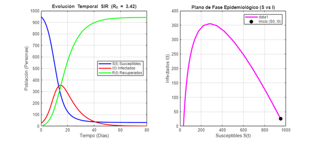
figure('Name', 'Modelo SIR Continuo - Análisis Dinámico', 'Position', [100 100 1000 450]);

subplot(1, 2, 1);
plot(xdata_sir, S_nom, 'b-', 'LineWidth', 2, 'DisplayName', 'S(t) Susceptibles');
hold on;
plot(xdata_sir, I_nom, 'r-', 'LineWidth', 2, 'DisplayName', 'I(t) Infectados');
plot(xdata_sir, R_nom, 'g-', 'LineWidth', 2, 'DisplayName', 'R(t) Recuperados');
xlabel('Tiempo (Días)');
ylabel('Población (Personas)');
title(sprintf('Evolución Temporal SIR (R_0 = %.2f)', R0_basic));
grid on;
legend('Location', 'east');

subplot(1, 2, 2);
plot(S_nom, I_nom, 'm-', 'LineWidth', 2.5);
hold on;
plot(S_nom(1), I_nom(1), 'ko', 'MarkerFaceColor', 'k', 'MarkerSize', 8, 'DisplayName', 'Inicio (S0, I0)');
xlabel('Susceptibles S(t)');
ylabel('Infectados I(t)');
title('Plano de Fase Epidemiológico (S vs I)');
grid on;
legend('Location', 'northeast');

% C. Muestreo de Ensamble para la Curva de Infectados (Salida 2)
T_sir.Properties.CustomProperties.output = 2; % Filtrar a Infectados (Salida 2)
M_sir = gsua_dmatrix(T_sir, 30);
Y_sir_ens = zeros(30, length(xdata_sir));
for i = 1:30
    Y_sir_ens(i,:) = gsua_eval(M_sir(i,:)', T_sir, xdata_sir, [], false, false, false);
end

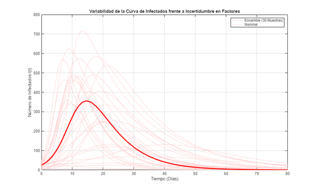
figure('Name', 'Modelo SIR - Variabilidad de Infectados');
plot(xdata_sir, Y_sir_ens', 'Color', [1.0 0.8 0.8], 'LineWidth', 0.8);
hold on;
plot(xdata_sir, I_nom, 'r-', 'LineWidth', 2.5, 'DisplayName', 'Nominal');
xlabel('Tiempo (Días)');
ylabel('Número de Infectados I(t)');
title('Variabilidad de la Curva de Infectados frente a Incertidumbre en Factores');
grid on;
legend('Ensamble (30 Muestras)', 'Nominal', 'Location', 'northeast');

--- 2. MODELO EPIDÉMICO SIR CONTINUO ---
Sistema EDO: dS/dt = -beta*S*I, dI/dt = beta*S*I - gamma*I, dR/dt = gamma*I

Setting environment to work with user-defined function
Tabla Resumen del Modelo SIR (Parámetros + Condiciones Iniciales):
                  Range          Nominal
             ________________    _______

    beta     0.0001    0.0008    0.00045
    gamma      0.05       0.2      0.125
    S0          900       999      949.5
    I0            1        50       25.5

Parámetros Nominales: beta = 0.00045, gamma = 0.12, S0 = 950
Número Reproductivo Básico Calculado: R0 = 3.42
-> R0 > 1: Existe brote epidémico (El número de infectados crece inicialmente).

4. PREGUNTAS Y EJERCICIOS PARA EL ESTUDIANTE

fprintf('=========================================================================\n');
fprintf('  PREGUNTAS DE ANÁLISIS Y EJERCICIOS DOCENTES  \n');
fprintf('=========================================================================\n');
fprintf('1. ¿Cómo cambia el tiempo de pico epidémico (t_max) cuando beta aumenta un 20%%?\n');
fprintf('2. Si el valor inicial I0 cambia de 1 a 50, ¿afecta el valor máximo del pico I_max?\n');
fprintf('3. En el modelo logístico discreto, ¿qué sucede con la trayectoria si r = 2.2?\n');
fprintf('=========================================================================\n\n');

=========================================================================
  PREGUNTAS DE ANÁLISIS Y EJERCICIOS DOCENTES  
=========================================================================
1. ¿Cómo cambia el tiempo de pico epidémico (t_max) cuando beta aumenta un 20%?
2. Si el valor inicial I0 cambia de 1 a 50, ¿afecta el valor máximo del pico I_max?
3. En el modelo logístico discreto, ¿qué sucede con la trayectoria si r = 2.2?
=========================================================================

Published with MATLAB® R2025b